Data Sources and Quality
Background
The main DesignBuilder Climate Analytics dataset is based on the Integrated Surface Database (ISD) which consists of global synoptic daily observations compiled from numerous sources into a single common format and data model. The data held in the ISD is checked by an extensive set of quality control algorithms for data validity, extreme values, internal consistency within observation, as well as external consistency with respect to other observations for the same station.
Design Year Data
Design Year data is based on measured daily min/max temperature, humidity, wind speed data recorded by weather stations combined with gridded data from the ISD. Specific weather station data has the advantage of considering local variations but it often has gaps or even missing years in the data series. Gridded data on the other hand usually has no gaps and the data is complete, but it does not always take into consideration local variations. Climate Analytics uses a wide range of statistical methods to combine weather station data with gridded data to include consideration of local variations but without the gaps normally associated with station data. To fill gaps in station data the tool uses various short term, medium term, long term , seasonal, yearly and long term deviation.
Behind the scenes, the daily max/min values are used to generate the hourly variations in solar radiation, temperature, wind etc required for the hourly weather files. For example, hourly Design Year temperature data is generated from daily min/max values stored in the database by fitting typical daily temperature profiles from the actual min/max value. Likewise, hourly solar values are calculated from the daily totals using standard daily profiles. The hourly variation of humidity is based on the most common local hourly variation over a year based on observations from the previous 40 years.
Design Temperature, wind, visibility and humidity data is mostly recorded by weather stations but all solar radiation data comes from gridded data built from a mix of ground station and satellite sources. All other variables that are not included in the station data come from grid data.
Note that the amount of data that comes from station measurements varies by country. The US and Norway are examples of countries that includes the most complete sets of measured daily data while Sweden is an example of a country that provides the minimum amount of measured data.
Actual Year Data
Actual Year data is obtained directly from a dense grid of hourly recorded values from NASA's MERRA2 reanalysis database. The spacial grid size is 0.5° latitude x 0.625° longitude with 72 pressure levels. For more information on the MERRA2 data see here and here.
Gridded Data
Design Year datasets also make extensive use of gridded data to fill in gaps in measured weather station values when they are missing. Gridded data is a mix of data from satellites, ground weather stations and radar and the selection of appropriate data is made upstream from Climate Analytics. The data comes from a wide range of data sources but mainly NOAA, NREL and satellite data which has been “smeared” over the surface of the globe.
Although raw gridded data is generally continuous (i.e. without gaps), it may include some degree of bias. For example temperatures may be consistently too high or low or the max/min range may not be accurate relative to station measurements. Climate Analytics corrects for any such bias by "morphing" the raw gridded data to fit with known maximum, minimum, average and range measurements from weather stations.
Gridded data is interpolated behind the scenes when necessary to obtain data for an exact point on the surface of the earth. For periods in the measured data where there are gaps, a check is made to see if there is a correspondence between the gridded and measured data and the gridded data is adjusted using various statistical methods to ensure that it fits well with measured data. Short hourly gaps, short-term daily gaps, daily and monthly long gaps or missing data each require a different method. In this way, gridded data is used to help plug any gaps in the measured data.
The grid distance intervals are different for the hourly NASA database used to create the Actual Year database and the daily NOAA database used to create the Design Year database. The NASA databases (used in Actual Year data) are based on a dense grid. For example, 4 grid points are provided for London whereas for the NOAA database (used in the Design Year data) interpolation is required behind the scenes to obtain a design year value inside city limits.
Summary of NOAA Daily vs NASA Hourly datasets
-
NOAA data is a mix of gridded and measured data and is used for daily totals and averages. Note that temperature is always measured and solar is always gridded. If temperature data is missing then all other data is also missing.
-
The coloured station data quality indicator icons apply specifically to Design daily data but they may also give a rough idea of Actual data quality too.
-
NASA data is used for Actual Year hourly values. The data is based on a dense grid, e.g. several points are provided within the London city limits whereas interpolation is required behind the scenes to obtain a design year value.
Data Quality
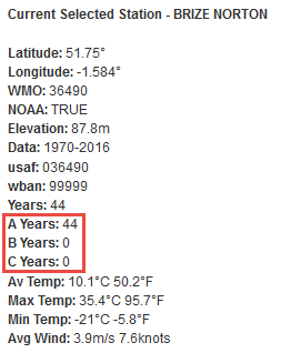
The design data for each station is classified for each year to define its quality. For example Heathrow and JFK airport have 365 days of measured design data available for all years and these are classified as Class A stations because gridded data is rarely required to fill gaps.
The system only uses stations where at least 80% measured data is available over 1-5 years so an extreme weather station in a remote region, which might produce couple of measured data points per year would be excluded from the listed stations. If not much measured data is available for a particular year, then more reliance is made on gridded data and the quality indicator will show data for that year to be Class C and accounted for in the summary statistics:
The specific definitions of A, B and C quality data are described on the Station tab help page.
The number of measured days of design data for each year can be viewed on the Analysis tab by choosing the "Yearly" interval and the Measured observations data. This output indicates the quality of the design data and hence the extent to which gridded data will be used to fill in gaps in measured data.
Some important points to note about the quality indicators are:
-
The quality indicator does not refer to Actual Year data which in general is of uniformly high quality.
-
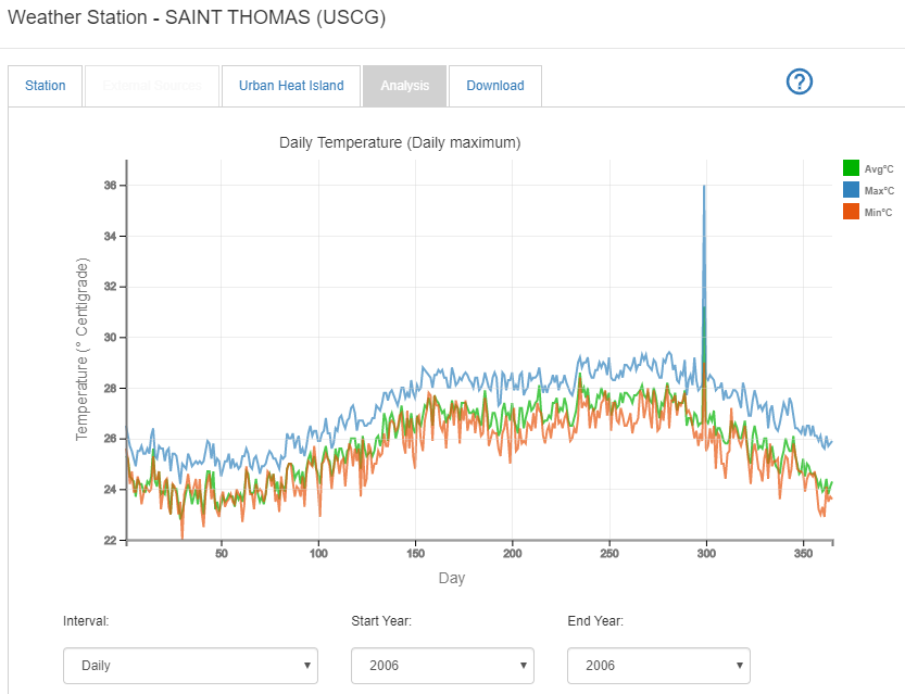
Even when measured data is available there can still be outliers and/or errors in the data. For example, the screenshot below shows that Saint Thomas has one day of maximum temperature 28.1⁰C on 25 Oct and the next day at 36.0⁰C deg. This outlier point could be caused by a day of freak weather, but it is also potentially an error. Climate Analytics does not change any of the original measured data, even if it could be wrong. It is left to the user to make selections by looking at all years and checking the minimum and maximum temperatures, wind speed etc to avoid particular years if necessary. It is therefore advisable to check data on the Analysis tab before downloading it for project work.
When using the of the “TRY” weather type options, this sort of data quality issue is less likely to be a concern because the TRY and TMY selection processes pick out the most typical Jan, Feb, March etc combining them together to make a year. Poor-quality data is unlikely to be selected as the most common and will be excluded. If you have one year where you notice unexpected data, you can simply select another year.
Data Modification and Morphing
A distinction is made between data modification and morphing and the differences between the 2 techniques is explained below.
Data modification
In the Climate Analytics context, data modification is a process where specific elements of recorded weather data are simply replaced by design values. For example:
Specific design sky conditions can be applied to model extreme design cases where clear skies or overcast skies or even completely dark skies are used in simulations to model worst case scenerios.
Likewise, specific design wind conditions can be applied. A common application is to use weather data with zero wind speed to access the performance of a building with natural ventilation under worst case conditions when air movement is driven only stack effect with no help from wind pressures.
Data morphing
In the Climate Analytics context, data morphing is a process where recorded weather data profiles are modified to account for known difference in time, space or situation. It goes beyond the simple "value swapping" approach used in data modification by transforming the data in a way that may result in different data shapes or representations. For example:
Future climate data is generated from recorded historical data by applying offsets derived from scenario analysis research projects. For most future scenarios, temperature changes are defined as monthly offsets with different values for day and night. Morphing algorithms are applied to ensure that these temperature offsets are applied so as to ensure a smooth transition from day to night and from month to month.
Urban heat island temperature offsets are also defined as different values for day and night using similar morphing algorithms as for future climate to ensure smooth day/night transitions.